Optimize Spark Joins Unfashionably

TL;DR —I optimized Spark joins and reduced runtime from 90 mins to just 7 mins. Use a withColumn operation instead of a join operation and optimize your Spark joins ~10 times faster.

If you are an experienced Spark developer, you have probably encountered the pain in joining dataframes. It is like you must be a true master to be able to join dataframes efficiently. The questions one may ask himself are:

• Should I repartition my dataframe?
• Should I broadcast the smaller dataframe?
• What about the spark.shuffle.partitions parameter?

These questions have been occupying many people for a long time. Some really nice rules of thumb were proposed over the years. A good rule of thumb and intuition help a lot in discovering what is the best method to perform a join, but nothing beats trial and error in my opinion.

I am about to present a really cool concept I developed while suffering tremendously from poor join performance.

What was I facing?

My primary data was a table with 300 columns and 200 million rows. About 100 columns were coded, and needed to be deciphered. We will call it DATA.

Luckily, I have another table, with translations to these codes. This table is much smaller — only 300k rows with a small number of columns. We will call it MAPPING.

MAPPING consists of one-to-one translations. For each value needed to be deciphered, there is only 1 value available as translation, with respect to its context. The context directs us on which translation of a code is to be used.

The naïve approach is using the Spark SQL API. We would iterate over the coded columns in DATA, and for each of those, we would find a translation in MAPPING.

More advanced approaches would have us playing with parameters (such as spark.shuffle.partitions) or trying to broadcast\repartition dataframes.

Either case, I was facing 100 join operations, and I didn’t like it.

Surprisingly— performing the naïve approach in my project took forever, about 90 minutes.
Keep scrolling and check out how I reduced it to 7 minutes.

Lets demonstrate

In this example, we are going to handle inventory data. We have several departments — hence a column named department_id. Each department has its own products — each of those products have product_id and product_name columns.

Here, the context is department_id, the coded column is product_id, and its translation is product_name.

Below is how MAPPING would look like.

Table 1

Now, we have a very large DB consists of orders of inventory items. DATA would look like this.

Table 2

All we would like to do in our processing, is to add the product_name column from MAPPING, to our data in DATA.

Now, lets have a look on how the naïve approach would look like:

Figure 1

In this example, we have only 1 column to be joined. In my use case, there are 200M rows and 100 columns of product_id — and each column needs to be joined on!

Usually a join will consume lots of networking for each join operation. Moreover, hashing\sorting will occur in order to complete a join operation. Anyway, we are talking about time expensive operations that slow down our processing.

Collect() is not a bad word

Working with databases helped me realize what I really wanted to have in my Spark application. I wanted an indexed join. Furthermore, DATA contained only a small number of values in the context column — leading me to think of partitioned tables.

I didn’t want spark to shuffle every time I joined these dataframes, I didn’t want spark to perform sorting for every column I tried to translate.

I literally pictured in my head how each dataframe row access a single DB partition, then uses the DB’s index, and retrieves its translation.

This led me to experiment joining dataframes with a dictionary.

What does it even mean?

Instead of joining 2 dataframes for 100 hundred times, I turned the join operation into a withColumn operation.

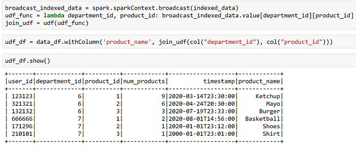
Let me remind you that MAPPING is a one-to-one translation. Leveraging this fact, we can create a user-defined-function (udf) that maps the coded value into a deciphered value.

Below you can see how to perform a withColumn join.
Later on I will discuss the obvious advantages using this kind of join.

First, we collect mapping_df into a hierarchical dictionary — the first hierarchy is department_id, and the second is product_id.

Figure 2

Then, we broadcast the dictionary, create a udf using the broadcasted dictionary, and join the values using the withColumn operation.

Figure 3

Now is the time to get in panic

Yes. I bet you could optimize your Spark pipeline’s join operations manyfold. I will now show a simple experiment proving this method to be of great value.

For the full experiment notebook, click here.

First, I created mapping_df, which contains 300K rows. We have 15 departments and 20K products per department.

Then, I created 2 dataframes — one for each join method, grouped by some columns, and executed the .count() action. The data in both dataframes is the same (both logically and practically — I validated it of course).
I ran the .count() action several times over each dataframe to get an average of the execution time.

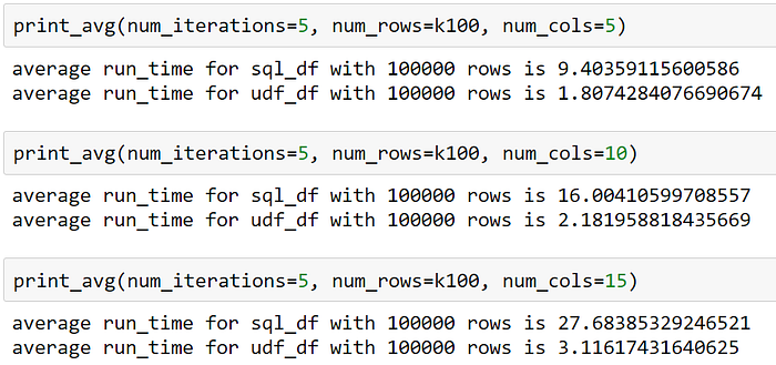
In the following experiment, I computed for the average run time for 5 runs. Here are some of my findings —

Figure 4

1. For a dataframe of 100K rows, we got better results using a withColumn join by up to 8.9 times faster than the naïve approach.
2. The higher the number of product_id columns to join on, the greater the relative difference between the executions was.
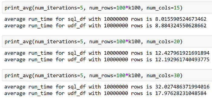
3. When we increased the number of rows (1M, 3M, 10M, 50M), and fixed the number of columns to join on (10), the relative difference between the run times decreased, as seen below.

Figure 5

“What about broadcast joins???”

That is a great question. Shouldn’t a regular broadcast join work better? It doesn’t involve UDFs and all the serialization problems. Looks like it should perform at least as good as a withColumn join.

You are absolutely right. Broadcast joins can work very good. In fact, they perform much better better when mapping_df is broadcasted first, and then used in the join operation to create sql_df.

But there is a but… :)

Below you can see the results for the experiment when mapping_df is broadcasted. It makes the action over sql_df much faster— 23 seconds without broadcasting for 10 columns compared to 12 seconds with broadcasting for 20 columns.

Figure 6

But what we do see, is that when the number of columns continues to increase, the withColumn approach takes the lead by far.

Our plans finally explained

Another major advantage of using an indexed join, is how the final execution plan looks like. It turns a plan which is un-understandable, into a plan which a novice Spark developer can handle.

Since a withColumn operation is somewhat equivalent to a select clause, Spark groups them all on the same stage, and therefore, all these “join” operations are executed in parallel.

On the other hand, since a join operation require a stage for itself, the joins are executed one after the other.

On the .explain() string, the withColumn operations appear on the same line, and doesn’t require additional stages to be executed (such as “Exchange “ — shuffling).
On the other hand, each join operation requires preliminary work — shuffling the data, sorting it, and only then joins it (for SortMergeJoin). This turns a simple join operation into a headache of a plan.

In extreme cases, such as when the number of columns is very large, Spark’s stack size could be overflowed and crash the application. This is due to a too long plan.

Conclusion

The withColumn approach worked very good for me, but it isn’t a magic trick one could apply to solve all problems.

When the number of columns to join is very large, this method could be very useful — but there is a tradeoff between the number of rows and number of columns. Be aware!

Magic tricks and rules of thumb can’t beat trial and error.

For me it works like a feedback loop.

1. Experimenting leads me to: better understanding and intuition, and greater knowledge.
2. My intuition lead me to propose such a method to solve my poor join performance.
3. Experimenting my intuition got me back to (1).

Thanks for reading.
Please comment and share use cases this method helped you with.

Acknowledgments — Yaniv Harpaz, for his great effort of helping me with Azure, for advising me when things weren’t going the way I thought they would, and for urging me to keep writing this article.

Footnote — Experiments Workspace

I worked with:

• Jupyter notebooks
• Azure’s HDInsight 4.0 (2 master nodes, 8 worker nodes — 16 cores and 112 GB RAM each)
• Pyspark — Spark 2.4 (2.4.5.4.1.1.2)
• Python 3.5.2